
Gradient Descent Algorithms
This post is about gradient descent algorithms and the different variants and optimizations that exist in order to make it converge faster or make it appropriate for certain environments.
Contents
Gradient Descent
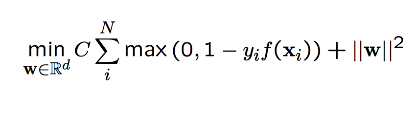
Gradient descent is classified as a first-order iterative optimization algorithm. It is an iterative process that on each iteration, it takes steps proportional to the negative of the gradient of the function we are trying to optimize (to find a local minimum). This family of algorithms can be used with classification methods such as Support Vector Machines. This is due to the fact that the cost function we are trying to minimize in Support Vector machines is convex and therefore local optimal points are globally optimal.
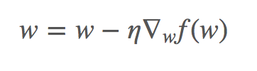
Vanilla Gradient Descent
The following is a simple implementation in python of the gradient descent method.
for t in range(n_iter):
for example in dataset: #for each point in our dataset
gradient = evaluate_gradient(loss_function, example, w) #compute the gradient
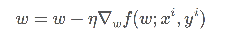
w = w - learning_rate * gradient #move in the negative gradient direction
– Visual representation of gradient descent Source
Projected Gradient Descent
If we are working with discrete data, it would be useful to change the code to make a projection of the gradient to a dataset point.
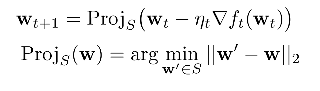
– This subtle change is what we call the projected gradient descent
Batch Gradient Descent
This variant is useful when we are processing several datapoints at a time. In batch gradient descent, we compute the gradient of the cost function w.
for t in range(n_iter):
  gradient = evaluate_gradient(loss_function, data, w) #compute the gradient
  w = w - learning_rate * gradient #move in the negative gradient direction
Stochastic Gradient Descent
We can see in the previous algorithm (batch descent) that we are performing operations with large matrices. We are performing several redundant operations as it recomputes gradients for similar examples.
Achieving Faster Convergence
After seeing the simple models, we know wish to accelerate the convergence. To do this, we may proceed using different methods.
- We could make stronger assumptions about our input data (see PEGASOS).
- We could adapt to the geometry of the input data (see AdaGrad).
PEGASOS
This method, first described by Shalev-Shwartz et al. 2007 assumes that the function on which we are working is H-strongly convex. Under these assumptions, we can see that the convergence happens faster.
Pseudocode:
#initialize w to a value so that:
#the norm of w <= 1/sqrt(lambda)

for t in range(n_iter):
  learning_rate = 1.0/np.sqrt(t*lambda)
  scalar = y[t]*np.dot(w.transpose(),x)
  #hinge loss for SVM
  loss = hinge_loss(y[t],x[t],scalar)
  if loss is not None:
     w = (1-learning_rate)*w - learning_rate*loss
  else:
     w *= (1-learning_rate)

  w *= min([1.0,1.0/(np.linalg.norm(w)*np.sqrt(lambda))])
ADAGRAD
Adagrad or Adaptive Gradient Algorithm is a method that adapts the learning rate to the input data. It performs larger updates for infrequent data and smaller updates for more frequent inputs.
Due to this, Adagrad is well suited for working with sparse datasets. Due to its nature, it will update more frequently the values with least probability.
For vanilla gradient descent, we perform an update for all parameters of w at once. And also, our learning rate was the same. Adagrad, however modifies the learning rate at set t based on past gradients. It keeps track of the past changes.
To store the past gradients, we will use a matrix G. This matrix at each step will be updated and extended.
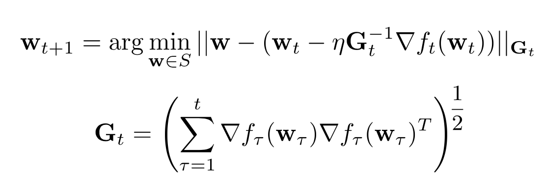 – Description of AdaGrad
This method, however, is very inefficient as it would require to compute a matrix multiplication and the square root of a matrix at each step.
Because of this, the general way of interpreting G is the following:
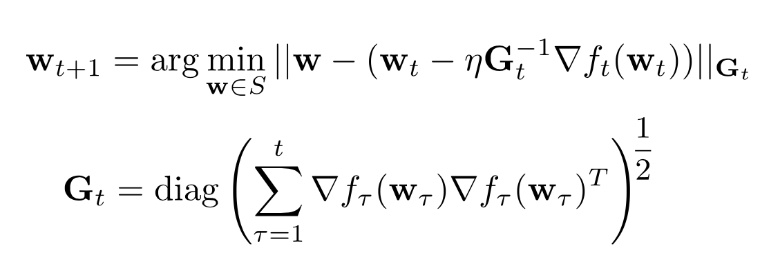 – Description of efficient AdaGrad
As we can see, now we only take into consideration the diagonal values of the matrix.
In the following image we can see a comparison of how several methods converge. As we can see in the image, Adagrad is one of the fastest and most “direct” methods as it adapts to the geometry of the data.
– Comparison of different methods Credit: Daniel Nouri
ADAM
This method described by Kingma & Lei Ba in 2014 3achieves faster convergence using moments. It is also a first-order gradient based and is very fast and memory efficient (no need to store a huge matrix like AdaGrad for example).
The method keeps in memory two arrays that correspond to the 1st moment and the 2nd moment. For each iteration, we compute the gradient and weight it according to both moments.
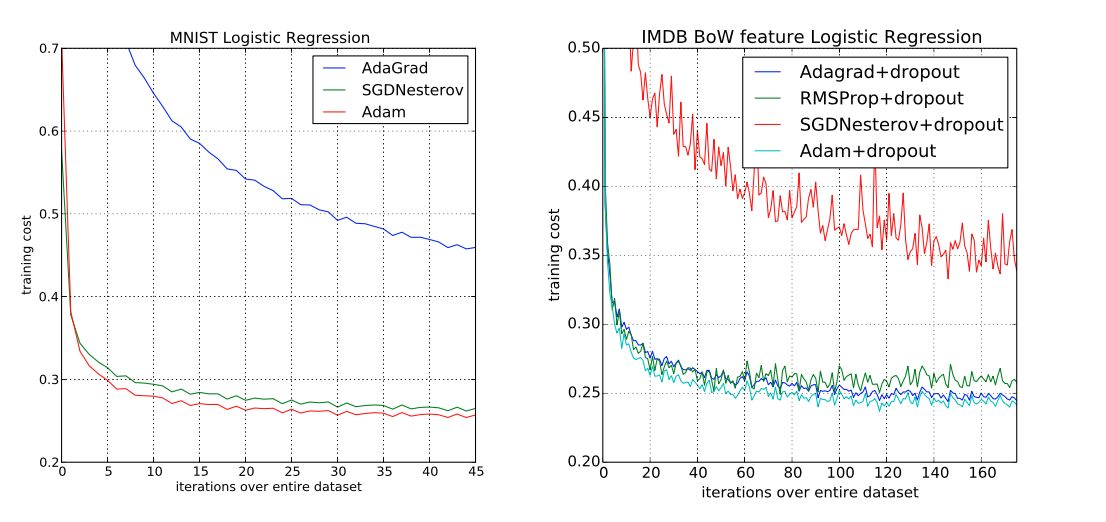
– Comparison in training cost (from Kingma & Lei Ba ‘14)
Parallel Methods for Distributed Environments
The previous discussed methods lets one train an SVM or a classifier one data point at a time without taking into in consideration issues about scalability.
What about massive data? For example, Streaming 2TB of data would take too long to compute. Also we would have to have a method that is light in memory due to the size of the data.
- Can we use these methods on a claster via Mapreduce?
- Can we use a multi-core system and exploit shared memory parallelism?
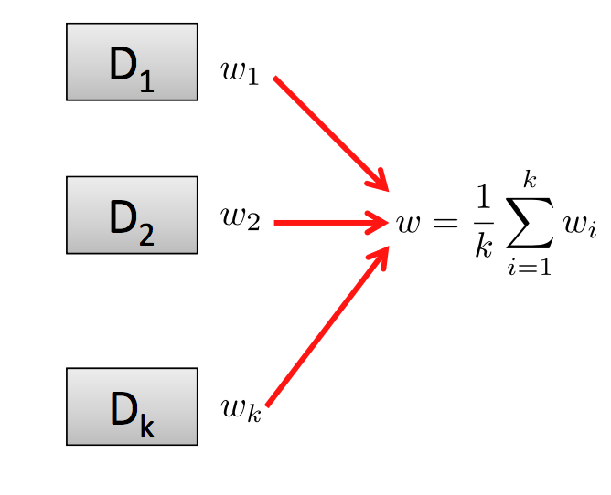
Parallel Stochastic Gradient Descent
This method proposed by Zinkevich et al 2010 makes a greedy assumption in order to exploit parallelism.
This method works extremely well in a Mapreduce environment. We split the initial dataset evenly over all the mappers. Each mapper outputs wi. The final reducer makes the greedy assumption that the final w is the average of all wi.
Shared memory parallelism - HogWild!
In order to achieve parallelism in a multi core machine, we would like to find a method that allows us to compute several gradient descents at the same time while keeping the shared w synchronized. How could we achieve this? We could lock w everytime we start a new thread in a core. However this would make the method very slow.
Niu, Recht, Re and Wright 2011 propose that we should not use any synchronization at all as long as data is sparse since each core would only access a small fraction of w. They show that it is unlikely that cores will overwrite relevant information in w when data is sparse.
– Layout of the system as described by Zinkevich et al. ‘11